Seaborn plot to visualize Iris data

I have created this Kernel for beginners who want to learn how to plot graphs with seaborn.This kernel is still a work in progress.I will be updating it further when I find some time.If you find my work useful please fo vote by clicking at the top of the page.Thanks for viewing

 [1]:

# This Python 3 environment comes with many helpful analytics libraries installed

# It is defined by the kaggle/python docker image: https://github.com/kaggle/docker-python

# For example, here's several helpful packages to load in 

​

import numpy as np # linear algebra

import pandas as pd # data processing, CSV file I/O (e.g. pd.read_csv)

​

# Input data files are available in the "../input/" directory.

# For example, running this (by clicking run or pressing Shift+Enter) will list the files in the input directory

​

import os

print(os.listdir("../input"))

​

# Any results you write to the current directory are saved as output.

['database.sqlite', 'Iris.csv']

Importing pandas and Seaborn module

 [2]:

import pandas as pd

import seaborn as sns

Importing Iris data set

 [3]:

iris=pd.read_csv('../input/Iris.csv')

Displaying data

 [4]:

iris.head()

[4]:

	Id	SepalLengthCm	SepalWidthCm	PetalLengthCm	PetalWidthCm	Species
0	1	5.1	3.5	1.4	0.2	Iris-setosa
1	2	4.9	3.0	1.4	0.2	Iris-setosa
2	3	4.7	3.2	1.3	0.2	Iris-setosa
3	4	4.6	3.1	1.5	0.2	Iris-setosa
4	5	5.0	3.6	1.4	0.2	Iris-setosa

 [5]:

iris.drop('Id',axis=1,inplace=True)

Checking if there are any missing values

 [6]:

iris.info()

<class 'pandas.core.frame.DataFrame'>
RangeIndex: 150 entries, 0 to 149
Data columns (total 5 columns):
SepalLengthCm    150 non-null float64
SepalWidthCm     150 non-null float64
PetalLengthCm    150 non-null float64
PetalWidthCm     150 non-null float64
Species          150 non-null object
dtypes: float64(4), object(1)
memory usage: 5.9+ KB

 [7]:

iris['Species'].value_counts()

[7]:

Iris-versicolor    50
Iris-setosa        50
Iris-virginica     50
Name: Species, dtype: int64

This data set has three varities of Iris plant.

Joint plot

 [8]:

sns.jointplot(x='SepalLengthCm',y='SepalWidthCm',data=iris,size=5)

[8]:

<seaborn.axisgrid.JointGrid at 0x7ff33a187e48>

FacetGrid Plot

 [9]:

import matplotlib.pyplot as plt

%matplotlib inline

sns.FacetGrid(iris,hue='Species',size=5)\

.map(plt.scatter,'SepalLengthCm','SepalWidthCm')\

.add_legend()

[9]:

<seaborn.axisgrid.FacetGrid at 0x7ff30ab847b8>

Boxplot

 [10]:

sns.boxplot(x='Species',y='PetalLengthCm',data=iris)

[10]:

<matplotlib.axes._subplots.AxesSubplot at 0x7ff306feaa58>

 

Strip plot

 [11]:

ax=sns.stripplot(x='Species',y='SepalLengthCm',data=iris,jitter=True,edgecolor='gray')

Combining Box and Strip Plots

 [12]:

ax=sns.boxplot(x='Species',y='SepalLengthCm',data=iris)

ax=sns.stripplot(x='Species',y='SepalLengthCm',data=iris,jitter=True,edgecolor='gray')

Violin Plot

 [13]:

sns.violinplot(x='Species',y='SepalLengthCm',data=iris,size=6)

[13]:

<matplotlib.axes._subplots.AxesSubplot at 0x7ff306e4ee48>

Pair Plot

 [14]:

sns.pairplot(data=iris,kind='scatter')

[14]:

<seaborn.axisgrid.PairGrid at 0x7ff306e702e8>

 [15]:

sns.pairplot(iris,hue='Species')

[15]:

<seaborn.axisgrid.PairGrid at 0x7ff324e57dd8>

Plotting heat map

 [16]:

plt.figure(figsize=(7,4))

sns.heatmap(iris.corr(),annot=True,cmap='summer')

[16]:

<matplotlib.axes._subplots.AxesSubplot at 0x7ff3043a1400>

Distribution plot

 [17]:

iris.hist(edgecolor='black', linewidth=1.2)

fig=plt.gcf()

fig.set_size_inches(12,6)

plt.show()

Swarm plot

 [18]:

sns.set(style="whitegrid")

fig=plt.gcf()

fig.set_size_inches(10,7)

fig = sns.swarmplot(x="Species", y="PetalLengthCm", data=iris)

PEARSON CORRELATION SCORE

Hello everyone, in our last Machine Learning tutorial we learnt about that how we can use Euclidean Distance formula to find out similarity among people. In this tutorial we learn a new way to do the same thing but in a bit complex or rather I should say in advanced manner. We will use Pearson Correlation Score for calculating similarity among people. It has one major difference in the result being generated by it, in comparison to Euclidean Distance, that even if the distance between the values of fruits provided by two persons is high, but if it is consistent, that is difference is nearly is consistent through out all fruits, then Pearson Correlation Score will mark both persons highly similar or totally same.

	Mango	Banana	Strawberry	Pineapple	Orange	Apple
John	4.5	3.5	4	4
Martha		2.5	4.5		5	3.5
Mathew	3.75		4.25	3		3.5
Nick	4	3		4.5	4.5

For example in the above data if we look at ‘John’ and ‘Martha’ the distance between the fruits between them is nearly same, as a result Pearson Correlation Value will be around ‘1’ for them.

We will calculate Pearson Correlation Score only for those fruits which are common for both the persons.

Above formula provides us the Pearson Correlation Coefficient or Score, where ‘n’ is the sample size or total number of fruits, ‘x’ and ‘y’ are the values corresponding to each fruit.

Python code for the above method:

 

#Dictionary of People rating for fruits choices={'John': {'Mango':4.5, 'Banana':3.5, 'Strawberry':4.0, 'Pineapple':4.0}, 'Nick': {'Mango':4.0, 'Orange':4.5, 'Banana':3.0, 'Pineapple':4.5}, 'Martha': {'Orange':5.0, 'Banana':2.5, 'Strawberry':4.5, 'Apple':3.5}, 'Mathew': {'Mango':3.75, 'Strawberry':4.25, 'Apple':3.5, 'Pineapple':3.0}} from math import sqrt #Finding Similarity among people using Eucledian Distance Formula class testClass():     def pearson(self, cho, per1, per2):         #Will set the following dictionary if data is common for two persons         sample_data={}         #Above mentioned varibale is an empty dictionary, that is length =0         for items in cho[per1]:             if items in cho[per2]:                 sample_data[items]=1                 #Value is being set 1 for those items which are same for both persons         #Calculating length of sample_data dictionary         length = len(sample_data)         #If both person does not have any similarity or similar items return 0         if length==0: return 0         #Remember one thing we will calculate all the below values only for common items         #   or the items which are being shared by both person1 and person2, that's why         #   we will be using sample_data dictionary in below loops         #Calculating Sum of all common elements for Person1 and Person2         sum1=sum([cho[per1][val] for val in sample_data])         sum2=sum([cho[per2][val] for val in sample_data])         #Calculating Sum of squares of all common elements for both         sumSq1=sum([pow(cho[per1][val],2) for val in sample_data])         sumSq2=sum([pow(cho[per2][val],2) for val in sample_data])         #Calculating Sum of Products of all common elements for both         sumPr=sum([cho[per1][val]*cho[per2][val] for val in sample_data])         #Calculating Person Correlation Score         x = sumPr-(sum1*sum2/length)         y = sqrt((sumSq1-pow(sum1,2)/length)*(sumSq2-pow(sum2,2)/length))         if y==0 : return 0         return(x/y)         #Value being returned above always lies between -1 and 1         #Value of 1 means maximum similarity def main():     ob = testClass()     print(ob.pearson(choices, 'John', 'Nick'))     print(ob.pearson(choices, 'John', 'Martha'))     print(ob.pearson(choices, 'John', 'John')) if __name__ == "__main__":     main()

RECOMMENDING ITEMS

Hi everyone in our last 2 tutorials we studied Eculidean Distance and Pearson Correlation Scorefor finding out similarity among people. Now its time to recommend some items to people which they have never tried.

Have you have ever thought that how different shopping websites or social media websites recommend items to us which we have never tried. Well there are multiple approaches, complex ones as well, to solve that problem, but at present we will look into one of the easiest ways for basic idea.

Approach for Recommending Items

	Mango	Banana	Strawberry	Pineapple	Orange	Apple
John	4.5	3.5	4	4
Martha		2.5	4.5		5	3.5
Mathew	3.75		4.25	3		3.5
Nick	4	3		4.5	4.5

We will use similarity score for finding out similarity among people, then we will check for the missing items for a person in comparison to others. Before I move on further in depth, lets take an example for better mapping. Using our above data-set we are required to recommend items to ‘John’.

1. Calculate similarity score of everyone with respect to ‘John’
2. Now list out items which others have provided rating but ‘John’ hasn’t.
3. We will use weighted rating for getting better result, that is, take product similarity score with each item, corresponding to other people.
   • In case of ‘Martha’, fruits which ‘John’ didn’t rate are Orange and Apple
   • Similarity score between ‘Martha’ and ‘John’ is ‘0.4721359549995794’
   • Weighted score = (Similarity_Score * Rating)
   • For Orange weighted score = 0.4721359549995794 * 5 = 2.360679774997897
   • Calculate weighted score corresponding to each fruit and for every other person.
4. Calculate sum of all the similarity scores corresponding to each other item
   • For Orange Sum of Similarity per Item (sspi) = Sum of Similarity Score of ‘Martha’ and ‘Nick’
     • sspi = 0.4721359549995794 + 0.5358983848622454
     • sspi = 1.008034339861825
   • For Apple Sum of Similarity per Item (sspi) = Sum of Similarity Score of ‘Martha’ and ‘Mathew’
     • sspi = 0.4721359549995794 + 0.439607805437114
     • sspi = 0.9117437604366934
5. Calculate Sum of Weighted Score per Item (swcpi)
   • For Orange swcpi = (Martha_Similarity_Score * Rating) + (Nick_Similarity_Score * Rating) 
     • swcpi = (0.4721359549995794 * 5) + (0.5358983848622454*4.5)
     • swcpi = 4.772222506878001
   • For Apple swcpi = 3.191103161528427
6. For better result we will take average of weighted score with respect to Sum of Similarity per Item.
   • For Orange Average Weighted Score (aws) = (Sum of Weighted Score per Item)/(Sum of Similarity per Item)
     • aws = (4.772222506878001) / (1.008034339861825)
     • aws = 4.734186444017519
   • For Apple Average Weighted Score (aws) = 3.5

The Ranking of fruits for John are equal to Average Weighted Score (aws)

Python implementation for above algorithm (here I have used Euclidea Distance formula for calculating similarity, you can use any other mathematical model as well, for doing the same like Pearson Correlation Score)

 

#Dictionary of People rating for fruits
choices={‘John’: {‘Mango’:4.5, ‘Banana’:3.5, ‘Strawberry’:4.0, ‘Pineapple’:4.0},
‘Nick’: {‘Mango’:4.0, ‘Orange’:4.5, ‘Banana’:3.0, ‘Pineapple’:4.5},
‘Martha’: {‘Orange’:5.0, ‘Banana’:2.5, ‘Strawberry’:4.5, ‘Apple’:3.5},
‘Mathew’: {‘Mango’:3.75, ‘Strawberry’:4.25, ‘Apple’:3.5, ‘Pineapple’:3.0}}

import pandas as pd

from math import sqrt

class testClass():
def create_csv(self):
df = pd.DataFrame.from_dict(choices, orient=’index’)
df.to_csv(‘fruits.csv’)

#Finding Similarity among people using Eucledian Distance Formula

def choice_distance(self, cho, per1, per2):
#Will set the following dictionary if data is common for two persons
sample_data={}
#Above mentioned varibale is an empty dictionary, that is length =0

for items in cho[per1]:
if items in cho[per2]:
sample_data[items]=1
#Value is being set 1 for those items which are same for both persons

#If both person does not have any similarity or similar items return 0
if len(sample_data)==0: return 0

#Calculating Euclidean Distance
final_sum = sum([pow(cho[per1][items]-cho[per2][items],2) for items in cho[per1] if items in cho[per2]])
return(1/(1+sqrt(final_sum)))
#Value being returned above always lies between 0 and 1
#Value 1 is added to sqrt to prevent 1/0 division and to normaloze result.

#Calculating similarity value for a person with repect to other people
def scoreForAll(self,cho,similarity=choice_distance):
for others in cho:
if others!=’John’:
score=similarity(self, cho, ‘John’, others),others
#Remember to add self keyword in above call
print(score)

#Recommending which fruit should a person try, which he or she has never tried
def recommendation(self, cho, per, sim_method=choice_distance):
sumS={}
total={}

for others in cho:
#Removing the comparison of the person to itself who needs recommendations.
if others==per: continue
similarVal=sim_method(self,cho,per,others)
if similarVal == 0: continue
#IF You Are Using Pearson Correlation Score then uncomment the below code
# and comment the line of code
#if similarVal<=0: continue

for fruits in cho[others]:
if fruits not in cho[per] or cho[per][fruits]==0:
#multiply similarity score with rating
total.setdefault(fruits,0)
total[fruits]+=cho[others][fruits]*similarVal

#calculate sum of similarities
sumS.setdefault(fruits,0)
sumS[fruits]+=similarVal

#Generating normalized data
result=[(totalVal/sumS[fruits],fruits) for fruits,totalVal in total.items()]
result.sort()
result.reverse()
return result

def main():

ob = testClass()
ob.create_csv()
ob.scoreForAll(choices)
print(ob.recommendation(choices,’John’))

if __name__ == “__main__”:
main()

 

Output :

 

(0.5358983848622454, 'Nick')

(0.4721359549995794, 'Martha')

(0.439607805437114, 'Mathew')

[(4.734186444017522, 'Orange'), (3.5, 'Apple')]

 

 

In out next tutorial I will come up with some new interesting techniques, to make you think how easy and interesting Machine Learning is!!

Stay tuned and keep learning!!

For more updates and news related to this blog as well as to data science, machine learning and data visualization.

 

Please Write Your Comments.

Thanks,

Rakesh Kumar

CREATING WORDS’ DATA-SET FROM RSS FEEDS

Hi Everyone!! Whenever we try to learn some Machine Learning algorithm, the first thing that comes to our mind is “How we can get live data or real data for testing our algorithm”. This article focuses on creating such data set only, by extracting data from RSS feeds of multiple websites. Just by adding the URL of different websites that use RSS feed, we will be able extract multiple words from them.

Advantage of doing so is, that we get an authentic data and we can use it for performing multiple Machine Learning algorithms like clustering or unsupervised learning and many more.

For enabling this functionality, I will be using ‘feedparser’ library of Python, its an open library which helps us to extract data from RSS feeds. You can easily download it for free!

Code for it is as follows:

 

#Import feedparser library and re (regular expression) library import feedparser import re #Creating dictionary of titles and word counts corresponding to a RSS feed def pullWordCount(url):     #Using feedparser to parse the feed     fed = feedparser.parse(url)     wordCount = {}     for x in fed.entries:         if 'summary' in x:             summary = x.summary         else:             summary = x.summary         #Extracting a list of words from feeds         diffWords = pullWords(x.title+ ' ' + summary)         for words in diffWords:             wordCount.setdefault(words, 0)             wordCount[words]+=1     return fed.feed.title,wordCount #Removing unnecessary data and refining our data def pullWords(htmlTag):     #removing all tags of html     txtData = re.compile(r']+>').sub('', htmlTag)     #split words with all the non-alpha characters     words = re.compile(r'[^A-Z^a-z]+').split(txtData)     #converting all the words to lower case, to create a uniformity     return [word.lower() for word in words if word!=''] #appearCount has number of times a word has appeared appearCount = {} #wordsCount has total words wordsCount = {} #testlist.txt contains URLs of websites for url in open('testlist.txt'):     title,wordC = pullWordCount(url)     wordsCount[title] = wordC     for word,count in wordC.items():         appearCount.setdefault(word,0)         if count>1:             appearCount[word]+=1 wordList=[] for wor,bc in appearCount.items():     percent=float(bc)/len('testlist.txt')     if percent>0.02 and percent<0.8:wordList.append(wor) #by above percentage we mean that we are using words which have appearance # percentage between 2% and 80%, you can modify it for different kind of results #our data will be saved in BlogWordsData.txt out=open('BlogWordsData.txt','w') out.write('TestingBlog') for word in wordList: out.write('\t%s' %word) out.write('\n') for blog,wc in wordsCount.items():     out.write(blog)     for word in wordList:         if word in wc: out.write('t%d' %wc[word])     else: out.write('\t0')     out.write('\n')

Test List (testlist.txt)

 

Output

In our next tutorial we will use the data extracted from same technique for learning some new techniques in Unsupervised Learning.

Stay tuned and keep learning!!

 

Please Write Your Comments.

Thanks,

Rakesh Kumar

 

FACE DETECTION USING OPENCV IN LIVE VIDEO

Hi learners!! We always come across the problem face detection in machine learning and we always jut think that how we can create a face detection algorithm in the easiest and fastest way. Well here is the answer! we will use OpenCV library of python for detecting faces in the live video being fed using your webcam. For initial level we are using this library but next time we will be creating our own model from scratch and will train it and then test it in real time!!

OpenCV

OpenCV is a library of python which supports a built in model for detecting faces in an image using Haar Cascades. We can use OpenCV for extracting frames from a video then we will apply Haar Cascade onto those frames and will create square on the face being present in image.

NOTE: Before moving onto the code you will be needed to download the “haarcascade_frontalface_default.xml” for running this face detection algorithm. You can find it here. This file basically contains weights for detecting faces

Code :

#importing OpenCV and Time library

import cv2

import time

#Reading data from the CSV file we downloaded

face_cascade = cv2.CascadeClassifier('C:/Documents/MachineLearning/haarcascade_frontalface_default.xml')

#Capturing Video from primary webcam, you can change number from 0 to any Integer

## for other webcams if you have many of them

cap = cv2.VideoCapture(0)

while (True):

#Reading frame from the live video feed

    ret, frame = cap.read()

#Converting frame into grayscale for better efficiency

    gray = cv2.cvtColor(frame, cv2.COLOR_BGR2GRAY)

#Using Haar Cascade for detecting faces in an image

    faces = face_cascade.detectMultiScale(gray, 1.3, 5)

#Creating the rectangle around face

    for (x,y,w,h) in faces:

        frame = cv2.rectangle(frame,(x,y),(x+w,y+h),(120,250,0),2)

#Displaying the captured frame in a window

    cv2.imshow('gray',frame)

#Applied 0.5 seconds delay such that a new frame will only be read every 0.5 seconds

#This decreases load on machine, because in general webcam captures 15 to 25 frames per second

    time.sleep(0.5)

    print("sleep done!!")

if cv2.waitKey(20) & 0xFF == ord('q'):

        break

cap.release()

cv2.destroyAllWindows(

 

 

 

 

Input – Output

      

 

The above algorithm was for starters!! In next tutorial we will be creating a face detection algorithm from scratch, then we will train it and use it!

Stay tuned for more learning!!

 

PLEASE WRITE YOUR COMMENTS.

THANKS,

RAKESH KUMAR

DATA CLEANING USING R

Introduction

While doing data data analysis, before analyzing the data for any kind of resultant, we most perform the most essential step, that is, Data Cleaning. Because when we get the data it may not be ready for complete analysis, like there might me missing values which will make our judgement wrong, outliers which may affect the Mean, Median; variable may spread across the values of a column (need to convert that column into multiple variables. i.e., columns) and many more. So before performing any kind of analysis for getting results by using any means like Linear Regression, we must do data cleaning for getting the accurate results.

Working on Data Set

Lets use one of the data-sets being provided in RStudio, that is, “SURVEY”. It consists of variables like “Age”, “Pulse rate”, “Gender(Sex)”, etc.

library(MASS)
View(survey)
head(survey, 10)

##       Sex Wr.Hnd NW.Hnd W.Hnd    Fold Pulse    Clap Exer Smoke Height
## 1  Female   18.5   18.0 Right  R on L    92    Left Some Never 173.00
## 2    Male   19.5   20.5  Left  R on L   104    Left None Regul 177.80
## 3    Male   18.0   13.3 Right  L on R    87 Neither None Occas     NA
## 4    Male   18.8   18.9 Right  R on L    NA Neither None Never 160.00
## 5    Male   20.0   20.0 Right Neither    35   Right Some Never 165.00
## 6  Female   18.0   17.7 Right  L on R    64   Right Some Never 172.72
## 7    Male   17.7   17.7 Right  L on R    83   Right Freq Never 182.88
## 8  Female   17.0   17.3 Right  R on L    74   Right Freq Never 157.00
## 9    Male   20.0   19.5 Right  R on L    72   Right Some Never 175.00
## 10   Male   18.5   18.5 Right  R on L    90   Right Some Never 167.00
##         M.I    Age
## 1    Metric 18.250
## 2  Imperial 17.583
## 3       16.917
## 4    Metric 20.333
## 5    Metric 23.667
## 6  Imperial 21.000
## 7  Imperial 18.833
## 8    Metric 35.833
## 9    Metric 19.000
## 10   Metric 22.333

summary(survey)

##      Sex          Wr.Hnd          NW.Hnd        W.Hnd          Fold    
##  Female:118   Min.   :13.00   Min.   :12.50   Left : 18   L on R : 99  
##  Male  :118   1st Qu.:17.50   1st Qu.:17.50   Right:218   Neither: 18  
##  NA's  :  1   Median :18.50   Median :18.50   NA's :  1   R on L :120  
##               Mean   :18.67   Mean   :18.58                            
##               3rd Qu.:19.80   3rd Qu.:19.73                            
##               Max.   :23.20   Max.   :23.50                            
##               NA's   :1       NA's   :1                                
##      Pulse             Clap       Exer       Smoke         Height     
##  Min.   : 35.00   Left   : 39   Freq:115   Heavy: 11   Min.   :150.0  
##  1st Qu.: 66.00   Neither: 50   None: 24   Never:189   1st Qu.:165.0  
##  Median : 72.50   Right  :147   Some: 98   Occas: 19   Median :171.0  
##  Mean   : 74.15   NA's   :  1              Regul: 17   Mean   :172.4  
##  3rd Qu.: 80.00                            NA's :  1   3rd Qu.:180.0  
##  Max.   :104.00                                        Max.   :200.0  
##  NA's   :45                                            NA's   :28     
##        M.I           Age       
##  Imperial: 68   Min.   :16.75  
##  Metric  :141   1st Qu.:17.67  
##  NA's    : 28   Median :18.58  
##                 Mean   :20.37  
##                 3rd Qu.:20.17  
##                 Max.   :73.00  
## 

 

Description of data-set is as follows:

Sex           <- The sex of the student (Factor with levels “Male” and “Female”.)
Wr.Hnd   <- span (distance from tip of thumb to tip of little finger of spread hand) of writing hand, in centimetres.
NW.Hnd  <- span of non-writing hand
W.Hnd     <- writing hand of student (Factor, with levels “Left” and “Right”.)
Fold          <- Fold your arms! Which is on top (Factor, with levels “R on L”, “L on R”, “Neither”.)
Pulse        <- pulse rate of student (beats per minute)
Clap         <- Clap your hands! Which hand is on top (Factor, with levels “Right”, “Left”, “Neither”.)
Exer        <- how often the student exercises (Factor, with levels “Freq” (frequently), “Some”, “None”.)
Smoke     <- how much the student smokes (Factor, levels “Heavy”, “Regul” (regularly), “Occas” (occasionally), “Never”.)
Height     <- height of the student in centimetres
M.I.           <- whether the student expressed height in imperial (feet/inches) or metric (centimetres/metres) units. (Factor, levels “Metric”, “Imperial”.)
Age          <- age of the student in years

By “View()” method above the data set opens separately in RStudio for better view and we can see the data type as well of each variable by hovering onto it.

By “summary()” we got the summary of data like “Min value”, “Max value”, “Mean”, “Frequency”, etc.

The main things that can be interpreted from above summary are:

1. Categorical Variables: Sex, W.Hnd, Fold, Clap, Exer, Smoke, M.I
2. Numerical Variables: Wr.Hnd, NW.Hnd, Pulse, Height, Age
3. Presence of “NA” –> which means that our data-set contains missing or undefined values. While visualising the data using View() we can verify that there are a lot of missing values.
4. Other factors like –> Frequecny in case of categorical variable and for Numeric variables we get Mean, Median, Min, Max, 1st and 3rd Quartile.

?? Now the first question would have aroused in your mind that if the data is missing then how we can do proper analysis of data. You would be thinking how we can rplace all “NA” with some data. For that we generally use Mean, Median and Mode.

Filling Up Missing Values:

Since we have worked upon the outliers now we can work upon the missing values. For removing the gaps in information we can replace “NA” with either “Mean”, “Median” or “Mode”, depending upon the scenarios.

Scenarios for Raplcaing Missing Values:

1. If variable is “Continuous” –> Replace NA with any either “Mean”, “Median” or “Mode”.
2. Otherwise

1. If data “Normally Distributed” –> Replace NA with “Mean”.
2. if data “Skewd” –> Replace NA with “Median”.

3. If “Categorical” –> Replace NA with “Mode”.

** For “Non-continuous Numerical” data we will be using “Histogram” to check distribution of data (Normal or Skewd).

Working on Survey Data-Set:

1. For variable “Sex” It is a Categorical variable so we will use Mode.

survey$Sex[is.na(survey$Sex)] <- "Female"
summary(survey$Sex)

## Female   Male 
##    119    118

2. For variable “Wr.Hnd” It is a Non-continuous Numerical Variable so first we will look for distribution of data, by using histogram.

hist(survey$Wr.Hnd, main="Wr.Hnd")

 

In above histogram we can see that the data is Right-Skewd, so we will replace “NA” with “Median”

survey$Wr.Hnd[is.na(survey$Wr.Hnd)] <- median(survey$Wr.Hnd, na.rm=TRUE)
summary(survey$Wr.Hnd)

##    Min. 1st Qu.  Median    Mean 3rd Qu.    Max. 
##   13.00   17.50   18.50   18.67   19.80   23.20

3. For variable “NW.Hnd” It is a Non-continuous Numerical Variable so first we will look for distribution of data, by using histogram.

hist(survey$NW.Hnd, main="NW.Hnd")

 

In above histogram we can see that the data is approximately “Right Skewd”, so we will replace “NA” with “Median”

survey$NW.Hnd[is.na(survey$NW.Hnd)] <- median(survey$NW.Hnd, na.rm=TRUE)
summary(survey$NW.Hnd)

##    Min. 1st Qu.  Median    Mean 3rd Qu.    Max. 
##   12.50   17.50   18.50   18.58   19.70   23.50

4. For variable “W.Hnd” It is a Categorical variable so we will use Mode.

survey$W.Hnd[is.na(survey$W.Hnd)] <- "Right"
summary(survey$W.Hnd)

##  Left Right 
##    18   219

5. For variable “Pulse” It is a Non-continuous Numerical Variable so first we will look for distribution of data, by using histogram.

hist(survey$Pulse, main="Pulse")

 

In above histogram we can see that the data is approximately “Normally Distributed”, so we will replace “NA” with “Mean”

survey$Pulse[is.na(survey$Pulse)] <- mean(survey$Pulse, na.rm=TRUE)
summary(survey$Pulse)

##    Min. 1st Qu.  Median    Mean 3rd Qu.    Max. 
##   35.00   68.00   74.15   74.15   80.00  104.00

6. For variable “Clap” It is a Categorical variable so we will use Mode.

survey$Clap[is.na(survey$Clap)] <- "Right"
summary(survey$Clap)

##    Left Neither   Right 
##      39      50     148

7. For variable “Smoke” It is a Categorical variable so we will use Mode.

survey$Smoke[is.na(survey$Smoke)] <- "Never"
summary(survey$Smoke)

## Heavy Never Occas Regul 
##    11   190    19    17

8. For variable “Height” It is a Non-continuous Numerical Variable so first we will look for distribution of data, by using histogram.

hist(survey$Height, main="Height")

 

In above histogram we can see that the data is approximately “Right Skewd”, so we will replace “NA” with “median”

survey$Height[is.na(survey$Height)] <- median(survey$Height, na.rm=TRUE)
summary(survey$Height)

##    Min. 1st Qu.  Median    Mean 3rd Qu.    Max. 
##   150.0   167.0   171.0   172.2   179.0   200.0

9. For variable “M.I” It is a Categorical variable so we will use Mode.

survey$M.I[is.na(survey$M.I)] <- "Metric"
summary(survey$M.I)

## Imperial   Metric 
##       68      169

summary(survey)

##      Sex          Wr.Hnd          NW.Hnd        W.Hnd          Fold    
##  Female:119   Min.   :13.00   Min.   :12.50   Left : 18   L on R : 99  
##  Male  :118   1st Qu.:17.50   1st Qu.:17.50   Right:219   Neither: 18  
##               Median :18.50   Median :18.50               R on L :120  
##               Mean   :18.67   Mean   :18.58                            
##               3rd Qu.:19.80   3rd Qu.:19.70                            
##               Max.   :23.20   Max.   :23.50                            
##      Pulse             Clap       Exer       Smoke         Height     
##  Min.   : 35.00   Left   : 39   Freq:115   Heavy: 11   Min.   :150.0  
##  1st Qu.: 68.00   Neither: 50   None: 24   Never:190   1st Qu.:167.0  
##  Median : 74.15   Right  :148   Some: 98   Occas: 19   Median :171.0  
##  Mean   : 74.15                            Regul: 17   Mean   :172.2  
##  3rd Qu.: 80.00                                        3rd Qu.:179.0  
##  Max.   :104.00                                        Max.   :200.0  
##        M.I           Age       
##  Imperial: 68   Min.   :16.75  
##  Metric  :169   1st Qu.:17.67  
##                 Median :18.58  
##                 Mean   :20.37  
##                 3rd Qu.:20.17  
##                 Max.   :73.00

By following the above process we raplaced all the missing values with some meaningful data, as you can see in the “summary()” of data there are no “NA”s. Now our data is much cleaner than the one we started with, and it looks good for further analysis. Now the next thing that we need to handle is “Outlier”

Outliers

Outliers are the data values which deviate a lot from most of the data values, either too big or too small in comparison to average values. Let us understand using an example…We will use “boxplot()” for finding the outliers.

#We will create it only for numeric variables not for categorical data

boxplot(survey$Wr.Hnd, main="Wr.Hnd")

 

boxplot(survey$NW.Hnd, main="NW.Hnd")

 

boxplot(survey$Pulse, main="Pulse")

 

boxplot(survey$Height, main="Height")

 

boxplot(survey$Age, main="Age")

 

From above boxplot of “survey” data-set we can see that for variables Wr.Hnd, NW.Hnd, Pulseand Age has got some dots or circles in the graph, either above or below the slim lines (called whiskers, 1st and 3rd Quartile of boxplot). Those circles represents the presence of outliers and number of outliers OR we can detect outliers in one more way, that is, all the values out of range of 5th and 95th percentile can be considered as Outlier.

Removing Outliers

We will use the second method for removing the outliers, because in case of boxplot we may endup loosing some crucial information too, as range being produced by the 1st and 3rd quartile is generally smaller in comparison to the range being produced by 5th and 95th percentile. For example:

1. Range generated by Quartiles

#For variable PULSE
## Range generated by Quartiles
## (-1.5 * IQR) to (1.5 * IQR), where (Inerquartile Range) IQR <- Q3 -Q1
#Q1 and Q3 are present in summary of Pulse, that we obtained at the beginning

Q3 <- 80
Q1 <- 66
IQR <- Q3 -Q1 
lower <- -1.5 * IQR
upper <- 1.5 * IQR

lower

## [1] -21

upper

## [1] 21

2. Range generated by 5th and 95th Percentiles

## Range generated by 5th and 95th Percentiles
## For this we use quantile(, ) method

lower <- quantile(survey$Pulse, 0.05, na.rm=TRUE)
upper <- quantile(survey$Pulse, 0.95, na.rm=TRUE)

lower

## 5% 
## 60

upper

## 95% 
##  92

So we can see the significant difference in the range of values. Thus we will be useing Percentile approach for capping the outliers. ** Another thing to be noted is that in case of Percentiles we are using level of significance, so per our requirement we can change it too. In general we use 5th and 95th percentiles.

After detecting outliers for a variable we will replace it with the Mean of the data. We will do the same procedure for all the variables containing outliers.

1. For variable Pulse

quantile(survey$Pulse, 0.05, na.rm=TRUE)

## 5% 
## 60

quantile(survey$Pulse, 0.95, na.rm=TRUE)

## 95% 
##  92

survey$Pulse <- ifelse(survey$Pulse > 92, 74.22, survey$Pulse)
survey$Pulse <- ifelse(survey$Pulse < 60, 74.22, survey$Pulse)

summary(survey$Pulse)

##    Min. 1st Qu.  Median    Mean 3rd Qu.    Max. 
##   60.00   70.00   74.15   74.25   78.00   92.00

boxplot(survey$Pulse, main="Pulse_Without_Outliers")

** So what happened here?? We are still able to see dots in boxplot!! Answer to this is though there are dots in boxplot, but we cann’t remove more data than that, because it will result in forging data, which will hamper the correct analysis of data. This happens a lot when you are working on large dataset, so keep in mind that not all the outliers can be removed

** Though if we don’t want them we can simply delete the data but it will result in data loss. So its not a good practice to delete them.

Now we will repeat same process for other three variables too.

2. For variable Wr.Hnd

quantile(survey$Wr.Hnd, 0.05, na.rm=TRUE)

## 5% 
## 16

survey$Wr.Hnd <- ifelse(survey$Wr.Hnd < 16, 18.84, survey$Wr.Hnd)

summary(survey$Wr.Hnd)

##    Min. 1st Qu.  Median    Mean 3rd Qu.    Max. 
##   16.00   17.50   18.60   18.84   19.80   23.20

boxplot(survey$Wr.Hnd, main="Wr.Hnd_Without_Outliers")

 

3. For variable NW.Hnd

quantile(survey$NW.Hnd, 0.05, na.rm=TRUE)

##   5% 
## 15.5

quantile(survey$NW.Hnd, 0.95, na.rm=TRUE)

##   95% 
## 22.22

survey$NW.Hnd <- ifelse(survey$NW.Hnd > 22.22, 18.53, survey$NW.Hnd)
survey$NW.Hnd <- ifelse(survey$NW.Hnd < 15.5, 18.53, survey$NW.Hnd)

summary(survey$NW.Hnd)

##    Min. 1st Qu.  Median    Mean 3rd Qu.    Max. 
##   15.50   17.50   18.50   18.52   19.50   22.20

boxplot(survey$NW.Hnd, main="NW.Hnd_Without_Outliers")

 

4. For variable Age

quantile(survey$Age, 0.95, na.rm=TRUE)

##     95% 
## 30.6836

survey$Age <- ifelse(survey$Age > 30.6836, 19.22, survey$Age)

summary(survey$Age)

##    Min. 1st Qu.  Median    Mean 3rd Qu.    Max. 
##   16.75   17.67   18.58   19.17   19.83   30.67

boxplot(survey$Age, main="Age_Without_Outliers")

 

This is the same scenario that we faced while removing outliers from variable Pulse, but here the number of outliers is high. So in this scenario you can omit the data containing outliers for better results.

That’s all for this lecture, in next lecture we look into the things in a much deeper way.

Keep Learning!!!

 

PLEASE WRITE YOUR COMMENTS.

THANKS,

RAKESH KUMAR

DISCRETE UNIFORM PROBABILITY DISTRIBUTION WITH MS-EXCEL

Hi ML enthusiasts! In our last post, we talked about basics of random variables, probability distributions and its types and how to generate a discrete probability distribution plot. In this article, we will talk about the Discrete Uniform Probability Distribution and its implementation with MS-Excel.

Discrete Uniform Probability Function

Consider the experiment of rolling a die. We have six possible outcomes in this case: 1, 2, 3, 4, 5, 6. Each outcome has equal chance of occurrence. Thus, the probability of getting a particular outcome is same, i.e., 1/6.

Consider the experiment of tossing a coin. We can have only two outcomes, Head and Tail. Also, for an unbiased coin, the probability of occurrence of each outcome is same, i.e., 1/2.

For an experiment having equally-likely outcomes and the number of outcomes being n, the probability of occurrence of each outcome becomes 1/n.

Thus, for uniform probability function, f(x) = 1/n.

Implementation using MS-Excel

Let’s see how to implement uniform probability distribution in MS-Excel now. Here, consider the case of rolling two dice. In this case, we get the following as outcomes:

(1,1), (1,2), …, (1,6), (2,1), (2,2), …, (2,6), (3,1), (3,2), …, (3,6), (4,1), (4,2), …, (4,6), (5,1), (5,2), …, (5,6), (6,1), (6,2), …, (6,6).

In this way, we get 6*6 = 36 outcomes. Since, the dice are unbiased, the outcomes will be equally likely. Thus, the probability of each outcome will be 1/36.

• To perform the analysis of probability curve on Excel, first make two columns and name them as outcomes and probabilities respectively.
• Now, select the rows of outcome column using ctrl+shift+down key and set the type as text, see screenshot below:

• Now, give the names of the outcomes as seen in the above screenshot. They signify the observations of your categorical variable, outcomes.
• Count the number of rows/outcomes by using the ROWS() function of excel. It returns the number of rows in a particular column or range. Select a separate cell in excel worksheet and type =ROWS(<your data range>) by selecting outcome the data column and then press enter.

• This will give you total number of outcomes, 36 in our case. Now, in the probability column, select one cell (C2). Type =1/$G$2 in it and then press enter. It gives the decimal value of 1/36. Drag the formula up to the last observation.

• Now, apply the sum() function to find if the total probability is 1.

• Select both the columns and their observation by ctrl+shift+down and then go to insert>scatter>scatter with only markers.

• Set axes labels, title of chart and legend location by going into layout tab. You will get a plot like the following screenshot shows:

You can make the same type of distribution curves with any experiment that produces equally-likely outcomes and have no bias in it. For example, tossing two coins, estimating the likelihood of drawing a particular card from a deck of cards etc. All of these are the examples which generate the uniform probability distributions. Since the data points are discrete in nature, the probability distribution curve will also be discrete.

So, with this we conclude our tutorial. In the next tutorial, we will talk about the concept of expected value, standard deviation, variance and binomial probability distribution.

 

Please Write Your Comments.

Thanks,

Rakesh Kumar

EXPECTED VALUE, VARIANCE AND STANDARD DEVIATION USING MS-EXCEL

Hi Everyone! Today,  we will learn about the concepts of expected value, variance and standard deviation. We will also learn about their implementation using MS-Excel.

Consider a firm M which has collected the data of profits and the probability of their occurrence. The profits can be taken in the scale of 1000’s of $. We will take this data for our further analysis.

Expected value

Expected value, or mean, can be defined as the measure of the central value of the random variable. It has the following formula.

Here, x is the value of random variable and f(x) is the values of probabilities of their occurrences. Thus, we can say that excepted value of x is the weighted average of the values of random variable with the weights as their probabilities. Please note that it is the central tendency of the random variable under consideration. It is not a hard-and-fast rule that it has to be the value which x assumes.

Implementation using MS-Excel

• The first step is to collect the data. The given data consists of two columns, x and f(x). Make the third column and given it the heading x*f(x).
• In the observation 1 of this third column, write the expression =<observation 1 of row x>*<observation 1 of f(x)> and then press enter.
• Drag the cell down to apply the formula for all the values of x.
• Now, apply the sum() function to all the observations of this third column and this gives the expected value or mean of x. To do this, select a cell. write =sum(<data>) and then press enter. For select the data, click on the first observation of third column, press ctrl+shift+down key and then press enter. This gives the E(x) value of x.

Variance and its implementation using MS-Excel

Variance can be defined as the measure of weighted average of square of deviation of random variable from its expected value or mean. The weights here are probabilities of x. The formula of variance is as follows:

To implement this function using excel, subtract mean from each value of x and then square it using ()^2 and then multiply each squared value with f(x). After this, find the total sum using the sum function.

Standard Deviation

It is the square root of variance. It gives us an estimate of how far are the values of random variable distributed from the mean.

Why square the differences?

For a random variable having values which are equally likely or having same probability of occurrence or f(x) being equal for each value of x, the values of x-µ being both positive and negative and with these values multiplied by f(x), when this product is summed up, the outcome will come out to be zero. That states, there is no deviation at all! But, that’s not true. Thus, we square the differences and then multiply those squared differences with f(x) and then find the square root of all the summed values. This gives us a better idea of standard deviation. The below image explains this phenomenon:

It is to be noted that if we don’t square the differences, the sum will come out to be zero.

So guys, with this we conclude our tutorial. In the next tutorial, we will learn about binomial probability distribution and its implementation using MS-Excel.

Please Write Your Comments.

Thanks,

Rakesh Kumar

MULTIVARIATE LINEAR REGRESSION WITH R

Hi ML Enthusiasts! Today, We will be learning how to perform multivariate linear regression using R.

We will be using a very famous data set “King County House sales” in which we will treat price as the dependent variable and other variables as independent variables. We will use these independent variables to predict the price of houses. Before going further, let’s know about our variables first.

The Dataset

In this data set, we have 19 house features and the number of observations being 21613.

–id: notation of the house

–date: date on which the house was sold

–price: price at which house was sold(target variable)

–bedrooms: number of bedrooms per house

–bathrooms: number of bathrooms per bedroom

–sqft_living: sqft footage of the home

–sqft_lot: sqft footage of the lot

–floors: total floors of the house

–waterfront: house which is having the waterfront view

–view: has been viewed

–condition: how good is the condition of the house

–grade: grade given to the house according to King County metrics

–sqft_above: apart from basement, sqft footage of the house

–yr_built: year in which the house was built

–yr_renovated: year in which house was renovated

–zipcode -lat: latitude coordinate

–long: longitude coordinate

–sqft_living15: living room area in 2015

–sqft_lot15: lot size area in 2015

Now, let’s read our csv file and store it in house dataframe and see if the data has any missing values.

house = read.csv('kc_house_data.csv')
summary(house)

##        id                         date           price        
##  Min.   :1.000e+06   20140623T000000:  142   Min.   :  75000  
##  1st Qu.:2.123e+09   20140625T000000:  131   1st Qu.: 321950  
##  Median :3.905e+09   20140626T000000:  131   Median : 450000  
##  Mean   :4.580e+09   20140708T000000:  127   Mean   : 540088  
##  3rd Qu.:7.309e+09   20150427T000000:  126   3rd Qu.: 645000  
##  Max.   :9.900e+09   20150325T000000:  123   Max.   :7700000  
##                      (Other)        :20833                    
##     bedrooms        bathrooms      sqft_living       sqft_lot      
##  Min.   : 0.000   Min.   :0.000   Min.   :  290   Min.   :    520  
##  1st Qu.: 3.000   1st Qu.:1.750   1st Qu.: 1427   1st Qu.:   5040  
##  Median : 3.000   Median :2.250   Median : 1910   Median :   7618  
##  Mean   : 3.371   Mean   :2.115   Mean   : 2080   Mean   :  15107  
##  3rd Qu.: 4.000   3rd Qu.:2.500   3rd Qu.: 2550   3rd Qu.:  10688  
##  Max.   :33.000   Max.   :8.000   Max.   :13540   Max.   :1651359  
##                                                                    
##      floors        waterfront            view          condition    
##  Min.   :1.000   Min.   :0.000000   Min.   :0.0000   Min.   :1.000  
##  1st Qu.:1.000   1st Qu.:0.000000   1st Qu.:0.0000   1st Qu.:3.000  
##  Median :1.500   Median :0.000000   Median :0.0000   Median :3.000  
##  Mean   :1.494   Mean   :0.007542   Mean   :0.2343   Mean   :3.409  
##  3rd Qu.:2.000   3rd Qu.:0.000000   3rd Qu.:0.0000   3rd Qu.:4.000  
##  Max.   :3.500   Max.   :1.000000   Max.   :4.0000   Max.   :5.000  
##                                                                     
##      grade          sqft_above   sqft_basement       yr_built   
##  Min.   : 1.000   Min.   : 290   Min.   :   0.0   Min.   :1900  
##  1st Qu.: 7.000   1st Qu.:1190   1st Qu.:   0.0   1st Qu.:1951  
##  Median : 7.000   Median :1560   Median :   0.0   Median :1975  
##  Mean   : 7.657   Mean   :1788   Mean   : 291.5   Mean   :1971  
##  3rd Qu.: 8.000   3rd Qu.:2210   3rd Qu.: 560.0   3rd Qu.:1997  
##  Max.   :13.000   Max.   :9410   Max.   :4820.0   Max.   :2015  
##                                                                 
##   yr_renovated       zipcode           lat             long       
##  Min.   :   0.0   Min.   :98001   Min.   :47.16   Min.   :-122.5  
##  1st Qu.:   0.0   1st Qu.:98033   1st Qu.:47.47   1st Qu.:-122.3  
##  Median :   0.0   Median :98065   Median :47.57   Median :-122.2  
##  Mean   :  84.4   Mean   :98078   Mean   :47.56   Mean   :-122.2  
##  3rd Qu.:   0.0   3rd Qu.:98118   3rd Qu.:47.68   3rd Qu.:-122.1  
##  Max.   :2015.0   Max.   :98199   Max.   :47.78   Max.   :-121.3  
##                                                                   
##  sqft_living15    sqft_lot15    
##  Min.   : 399   Min.   :   651  
##  1st Qu.:1490   1st Qu.:  5100  
##  Median :1840   Median :  7620  
##  Mean   :1987   Mean   : 12768  
##  3rd Qu.:2360   3rd Qu.: 10083  
##  Max.   :6210   Max.   :871200  
## 

As can be seen from above details, there are no missing values, so there is no need to do missing value imputation. We can proceed towards our data relationship analysis. Now, let’s see how our data looks like by using the head() function.

head(house)

##           id            date   price bedrooms bathrooms sqft_living
## 1 7129300520 20141013T000000  221900        3      1.00        1180
## 2 6414100192 20141209T000000  538000        3      2.25        2570
## 3 5631500400 20150225T000000  180000        2      1.00         770
## 4 2487200875 20141209T000000  604000        4      3.00        1960
## 5 1954400510 20150218T000000  510000        3      2.00        1680
## 6 7237550310 20140512T000000 1225000        4      4.50        5420
##   sqft_lot floors waterfront view condition grade sqft_above sqft_basement
## 1     5650      1          0    0         3     7       1180             0
## 2     7242      2          0    0         3     7       2170           400
## 3    10000      1          0    0         3     6        770             0
## 4     5000      1          0    0         5     7       1050           910
## 5     8080      1          0    0         3     8       1680             0
## 6   101930      1          0    0         3    11       3890          1530
##   yr_built yr_renovated zipcode     lat     long sqft_living15 sqft_lot15
## 1     1955            0   98178 47.5112 -122.257          1340       5650
## 2     1951         1991   98125 47.7210 -122.319          1690       7639
## 3     1933            0   98028 47.7379 -122.233          2720       8062
## 4     1965            0   98136 47.5208 -122.393          1360       5000
## 5     1987            0   98074 47.6168 -122.045          1800       7503
## 6     2001            0   98053 47.6561 -122.005          4760     101930

The date variable needs our attention here. It’s in incorrect format. Let’s convert it in a UTC format using lubridate library.

#The date may not be in character data type. So, we use as.character() 
#in this case andsubset the date string with start=1 and stop = 8
house$date <- as.character(house$date)
house$date <- substr(house$date, 1, 8) 
#Convert the date in year-month-date format
house$date <- as.Date(house$date, , format='%Y%m%d')
#Converting date into number of days with 1st jan 1900 as reference date
house$date <- as.numeric(as.Date(house$date, origin = "1900-01-01"))
head(house)

##           id  date   price bedrooms bathrooms sqft_living sqft_lot floors
## 1 7129300520 16356  221900        3      1.00        1180     5650      1
## 2 6414100192 16413  538000        3      2.25        2570     7242      2
## 3 5631500400 16491  180000        2      1.00         770    10000      1
## 4 2487200875 16413  604000        4      3.00        1960     5000      1
## 5 1954400510 16484  510000        3      2.00        1680     8080      1
## 6 7237550310 16202 1225000        4      4.50        5420   101930      1
##   waterfront view condition grade sqft_above sqft_basement yr_built
## 1          0    0         3     7       1180             0     1955
## 2          0    0         3     7       2170           400     1951
## 3          0    0         3     6        770             0     1933
## 4          0    0         5     7       1050           910     1965
## 5          0    0         3     8       1680             0     1987
## 6          0    0         3    11       3890          1530     2001
##   yr_renovated zipcode     lat     long sqft_living15 sqft_lot15
## 1            0   98178 47.5112 -122.257          1340       5650
## 2         1991   98125 47.7210 -122.319          1690       7639
## 3            0   98028 47.7379 -122.233          2720       8062
## 4            0   98136 47.5208 -122.393          1360       5000
## 5            0   98074 47.6168 -122.045          1800       7503
## 6            0   98053 47.6561 -122.005          4760     101930

Our next step is to split the dataset into training and test data set. We do this by using the sample() function of R. We fix the ratio of training to test data as 80:20. So, we convert 0.2xdataset into test data and use the remaining, i.e., 0.8xdataset as training dataset.

splitRatio = sample(1:nrow(house), 0.2*nrow(house))
testHouseData = house[splitRatio,]
trainingHouseData = house[-splitRatio,]

Now comes the visualization part. Let’s look at how different variables are connected to price variable.

library(ggplot2)
library(GGally)
relPlot1 <- ggpairs(data = trainingHouseData, 
                    columns = 3:7,
                    mapping = aes(color = "dark green"),
                    axisLabels = "show")
relPlot1

One thing to be noted above is that all the columns from 3 to 7 are having continuous numerical data. So, the columns = 3:7 has been fixed. After 7th column, all the columns from 8 to 12 are categorical in nature. So, we use columns = c(3, 8:12) with 3rd column(price) having continuous numerical data.

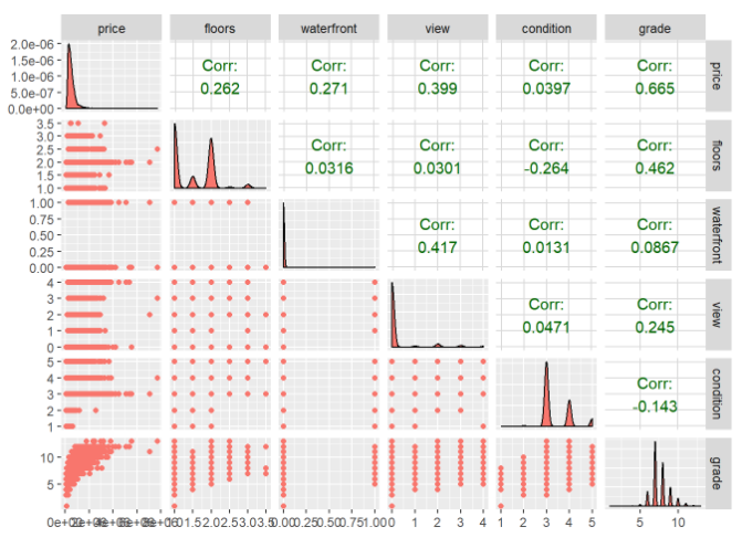
relPlot2 <- ggpairs(data = trainingHouseData, 
                    columns = c(3, 8:12),
                    mapping = aes(color = "dark green"),
                    axisLabels = "show")
relPlot2

Let’s verify the relationship between columns 3, 15, 18 and 19.

relPlot3 <- ggpairs(data = trainingHouseData, 
                    columns = c(3, 15, 18, 19),
                    mapping = aes(color = "dark green"),
                    axisLabels = "show")
relPlot3

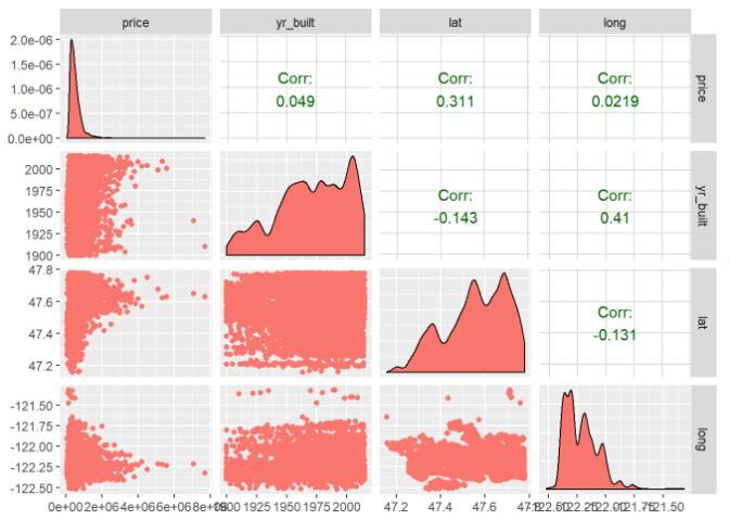
As you can see from the above plots, -corr between price vs sqft_living: 0.701 -corr between price vs bathrooms: 0.524 -corr between price vs grade: 0.654 -corr between price vs view: 0.406 -corr between price vs waterfront: 0.324 -corr between price vs lat: 0.304 -corr between price vs bedrooms: 0.303 -corr between price vs floors: 0.282 The correlation values between price and other variables are very small so that can be ignored as they are not posing any impact on the prices of the houses. Let’s now check the multi-collinearity among the variables using variance inflation factor concept.

library(car)

## Loading required package: carData

finalModel <- lm(price~sqft_living + bathrooms + grade + view + waterfront + bedrooms + floors, data=trainingHouseData)
vif(finalModel)

## sqft_living   bathrooms       grade        view  waterfront    bedrooms 
##    3.906712    2.858481    2.733885    1.321960    1.214251    1.609194 
##      floors 
##    1.451042

Since all the vif values are less than 5, we can say that the model doesn’t have multicollinearity among the variables. So, we can consider all the variables of the said model.

step(finalModel)

## Start:  AIC=427290.6
## price ~ sqft_living + bathrooms + grade + view + waterfront + 
##     bedrooms + floors
## 
##               Df  Sum of Sq        RSS    AIC
##                       9.3237e+14 427291
## - bathrooms    1 7.6493e+11 9.3314e+14 427303
## - floors       1 2.0967e+12 9.3447e+14 427327
## - bedrooms     1 7.3436e+12 9.3971e+14 427424
## - view         1 3.5588e+13 9.6796e+14 427936
## - waterfront   1 3.6058e+13 9.6843e+14 427945
## - grade        1 8.4533e+13 1.0169e+15 428789
## - sqft_living  1 1.3231e+14 1.0647e+15 429583

## 
## Call:
## lm(formula = price ~ sqft_living + bathrooms + grade + view + 
##     waterfront + bedrooms + floors, data = trainingHouseData)
## 
## Coefficients:
## (Intercept)  sqft_living    bathrooms        grade         view  
##   -468540.7        189.5     -14629.0      98753.5      68512.7  
##  waterfront     bedrooms       floors  
##    561511.0     -27997.1     -24612.7

According to the above stats, our finalModel equation is price = 191.1(sqft_living) – 13159.1(bathrooms) + 98298.6(grade)+66911.4(view) +580801.6(waterfront) – 27495.8(bedrooms) – 27293.2(floors) – 467519.7. Let’s find out what is the value of R-square of this model by using summary() function.

summary(finalModel)

## 
## Call:
## lm(formula = price ~ sqft_living + bathrooms + grade + view + 
##     waterfront + bedrooms + floors, data = trainingHouseData)
## 
## Residuals:
##      Min       1Q   Median       3Q      Max 
## -1186479  -125387   -18824    95760  4742318 
## 
## Coefficients:
##               Estimate Std. Error t value Pr(>|t|)    
## (Intercept) -4.685e+05  1.553e+04 -30.164  < 2e-16 ***
## sqft_living  1.895e+02  3.826e+00  49.523  < 2e-16 ***
## bathrooms   -1.463e+04  3.885e+03  -3.766 0.000167 ***
## grade        9.875e+04  2.495e+03  39.585  < 2e-16 ***
## view         6.851e+04  2.668e+03  25.684  < 2e-16 ***
## waterfront   5.615e+05  2.172e+04  25.853  < 2e-16 ***
## bedrooms    -2.800e+04  2.400e+03 -11.667  < 2e-16 ***
## floors      -2.461e+04  3.948e+03  -6.234 4.64e-10 ***
## ---
## Signif. codes:  0 '***' 0.001 '**' 0.01 '*' 0.05 '.' 0.1 ' ' 1
## 
## Residual standard error: 232300 on 17283 degrees of freedom
## Multiple R-squared:  0.5901, Adjusted R-squared:  0.5899 
## F-statistic:  3554 on 7 and 17283 DF,  p-value: < 2.2e-16

From above summary, we can say R-square is 59.72% or about 59.72% of variation in prices is explained by our chosen variables. Let’s work on increasing the accuracy of model by eliminating bedrooms and floors.

finalModel2 <- lm(price~sqft_living + bathrooms + grade + view + waterfront, data=trainingHouseData)
vif(finalModel2)

## sqft_living   bathrooms       grade        view  waterfront 
##    3.279054    2.447752    2.482267    1.303474    1.210474

Again, all the vif values are less than 5. So, we incorporate all the variables.

step(finalModel2)

## Start:  AIC=427451.8
## price ~ sqft_living + bathrooms + grade + view + waterfront
## 
##               Df  Sum of Sq        RSS    AIC
##                       9.4132e+14 427452
## - bathrooms    1 3.8429e+12 9.4516e+14 427520
## - waterfront   1 3.7003e+13 9.7832e+14 428116
## - view         1 3.9994e+13 9.8131e+14 428169
## - grade        1 9.5435e+13 1.0368e+15 429120
## - sqft_living  1 1.3552e+14 1.0768e+15 429775

## 
## Call:
## lm(formula = price ~ sqft_living + bathrooms + grade + view + 
##     waterfront, data = trainingHouseData)
## 
## Coefficients:
## (Intercept)  sqft_living    bathrooms        grade         view  
##   -548057.1        175.7     -30342.4      99983.0      72120.9  
##  waterfront  
##    567935.6

The equation in this case becomes price = 178.1(sqft_living) – 29722.6(bathrooms) + 98868.0(grade) + 70679.4(view) +588863.0(waterfront)-544112.4. Let’s now find out the R square of this model.

summary(finalModel2)

## 
## Call:
## lm(formula = price ~ sqft_living + bathrooms + grade + view + 
##     waterfront, data = trainingHouseData)
## 
## Residuals:
##      Min       1Q   Median       3Q      Max 
## -1200221  -125937   -18891    97404  4857478 
## 
## Coefficients:
##               Estimate Std. Error t value Pr(>|t|)    
## (Intercept) -5.481e+05  1.390e+04  -39.44   <2e-16 ***
## sqft_living  1.757e+02  3.522e+00   49.88   <2e-16 ***
## bathrooms   -3.034e+04  3.612e+03   -8.40   <2e-16 ***
## grade        9.998e+04  2.388e+03   41.86   <2e-16 ***
## view         7.212e+04  2.661e+03   27.10   <2e-16 ***
## waterfront   5.679e+05  2.179e+04   26.07   <2e-16 ***
## ---
## Signif. codes:  0 '***' 0.001 '**' 0.01 '*' 0.05 '.' 0.1 ' ' 1
## 
## Residual standard error: 233400 on 17285 degrees of freedom
## Multiple R-squared:  0.5861, Adjusted R-squared:  0.586 
## F-statistic:  4896 on 5 and 17285 DF,  p-value: < 2.2e-16

As you can see, the R square is nearly the same but our model has less variable dependency now. Also, since the P value of all the variables is less than 0.05, we reject the null hypothesis that there is no relationship among a particular variable and price and accept the alternate hypothesis that the price is dependent upon all the given variables. Now, let’s see if the assumptions of linear regression are satisfied or not.

library(lmtest)

## Loading required package: zoo

## 
## Attaching package: 'zoo'

## The following objects are masked from 'package:base':
## 
##     as.Date, as.Date.numeric

par(mfrow=c(2,2))
plot(finalModel2)

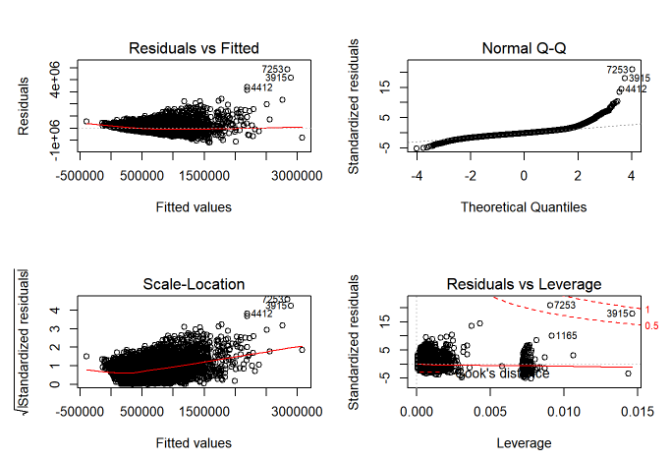
According to the assumptions of linear regression, these graphs must be uniformly distributed but that is not so here. So, we need to improve our model. Let’s now use our second model to predict the price for test dataset.

quantile(trainingHouseData$price, seq(0, 1, 0.01))

##        0%        1%        2%        3%        4%        5%        6% 
##   75000.0  153000.0  175000.0  190954.4  202500.0  210000.0  219970.0 
##        7%        8%        9%       10%       11%       12%       13% 
##  226465.0  234000.0  240000.0  246000.0  250000.0  255000.0  260000.0 
##       14%       15%       16%       17%       18%       19%       20% 
##  266500.0  270975.0  276000.0  280000.0  287000.0  291510.0  299000.0 
##       21%       22%       23%       24%       25%       26%       27% 
##  300000.0  306500.0  311925.0  317000.0  322000.0  325000.0  330000.0 
##       28%       29%       30%       31%       32%       33%       34% 
##  335000.0  340000.0  346000.0  350000.0  355000.0  360000.0  365042.0 
##       35%       36%       37%       38%       39%       40%       41% 
##  370975.0  375000.0  380500.0  388500.0  394905.0  399950.0  402000.0 
##       42%       43%       44%       45%       46%       47%       48% 
##  410000.0  415000.0  420000.0  425000.0  430000.0  436000.0  440000.0 
##       49%       50%       51%       52%       53%       54%       55% 
##  449000.0  450000.0  458000.0  465000.0  470000.0  475799.4  483972.5 
##       56%       57%       58%       59%       60%       61%       62% 
##  490000.0  499000.0  501000.0  510000.0  520000.0  525000.0  533040.0 
##       63%       64%       65%       66%       67%       68%       69% 
##  540000.0  548000.0  550060.0  560000.0  569000.0  575555.0  585000.0 
##       70%       71%       72%       73%       74%       75%       76% 
##  595000.0  603500.0  615000.0  625000.0  635000.0  645000.0  654000.0 
##       77%       78%       79%       80%       81%       82%       83% 
##  665000.0  678020.0  690000.0  700500.0  718500.0  732000.0  749997.8 
##       84%       85%       86%       87%       88%       89%       90% 
##  762000.0  780000.0  799080.0  815000.0  838000.0  860000.0  889000.0 
##       91%       92%       93%       94%       95%       96%       97% 
##  917450.0  950000.0  994970.0 1059800.0 1150000.0 1250000.0 1378600.0 
##       98%       99%      100% 
## 1595000.0 1959100.0 7700000.0

As you can see, there are outliers in the above price variable. So, we need to perform outlier handling.

trainingHouseData_new = trainingHouseData
trainingHouseData_new$price = ifelse(trainingHouseData_new$price>=1959100.0, 1959100.0, trainingHouseData_new$price)
trainingHouseData_new$price = ifelse(trainingHouseData_new$price<=155000.0, 155000.0, trainingHouseData_new$price)
finalModel3 <- lm(price~sqft_living + bathrooms + grade + view + waterfront+ bedrooms + floors, data=trainingHouseData_new)
summary(finalModel3)

## 
## Call:
## lm(formula = price ~ sqft_living + bathrooms + grade + view + 
##     waterfront + bedrooms + floors, data = trainingHouseData_new)
## 
## Residuals:
##     Min      1Q  Median      3Q     Max 
## -970881 -120334  -19718   90945 1220350 
## 
## Coefficients:
##               Estimate Std. Error t value Pr(>|t|)    
## (Intercept) -4.662e+05  1.327e+04 -35.144  < 2e-16 ***
## sqft_living  1.465e+02  3.268e+00  44.822  < 2e-16 ***
## bathrooms   -1.608e+04  3.318e+03  -4.847 1.26e-06 ***
## grade        1.026e+05  2.131e+03  48.145  < 2e-16 ***
## view         6.690e+04  2.278e+03  29.362  < 2e-16 ***
## waterfront   3.265e+05  1.855e+04  17.602  < 2e-16 ***
## bedrooms    -1.567e+04  2.049e+03  -7.644 2.22e-14 ***
## floors      -1.479e+04  3.372e+03  -4.386 1.16e-05 ***
## ---
## Signif. codes:  0 '***' 0.001 '**' 0.01 '*' 0.05 '.' 0.1 ' ' 1
## 
## Residual standard error: 198400 on 17283 degrees of freedom
## Multiple R-squared:  0.6047, Adjusted R-squared:  0.6046 
## F-statistic:  3778 on 7 and 17283 DF,  p-value: < 2.2e-16

Thus, the R square has improved to 61.07%. Let’s now do the assumptions analysis.

par(mfrow=c(2,2))
plot(finalModel3)

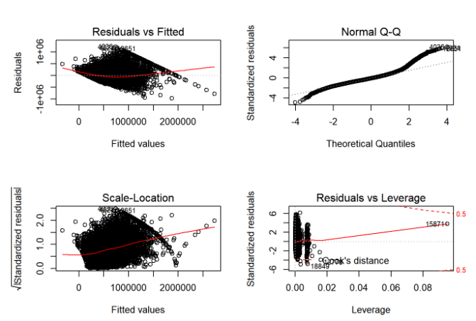
Thus, with outlier manipulation, the residuals vs leverage quality has dropped but quality for other graphs has improved. Also, now 61.07% of variation in price can be explained by the other independent variables in the model. Let’s now apply durbin watson test to our model.

durbinWatsonTest(finalModel3)

##  lag Autocorrelation D-W Statistic p-value
##    1       0.0131114      1.973754    0.09
##  Alternative hypothesis: rho != 0

The DW statistic is 1.978 or approximately 2. Thus, there is no autocorrelation among the variables. Hence, all the assumptions of linear regression are satisfied.

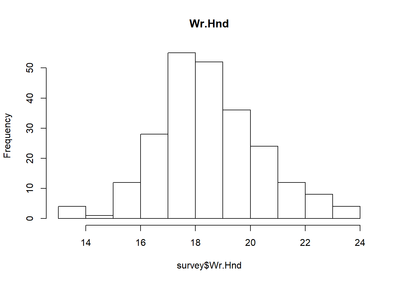
hist(residuals(finalModel3))

 The histogram of residuals is also coming out to be approximately normal which is a positive indication.Now, let’s check for homoscedasticity.

plot(trainingHouseData_new$price, residuals(finalModel3))

The distribution is uniform in nature which is another positive indication. Now, let’s do the prediction.

testHouseData$predictedPrice = predict(finalModel3, testHouseData)

 

Please Write Your Comments.

Thanks,

Rakesh Kumar

THE MATHEMATICS BEHIND UNIVARIATE LINEAR REGRESSION

Hi ML Enthusiasts! Today, we are going to learn about the mathematics behind linear regression.

Basics of Linear Regression

The equation or curve that is used to represent the linear law is given as below:

where i ranges from 1 to number of observations, N,

y_i is the output variable, also called as predicted variable in Machine Learning terms,

x_i is the input or explanatory variable,

m is defined as the slope or differential change in the value of y due to differential change in x,

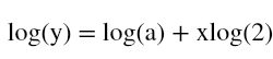
 and in case of multiple input variables or features,

and, c is called as intercept in mathematical terms. It can also be described as the variation in predicted value which can’t be explained by x or the input variable(s).

The above equation predicts value of y for each value of x.

The Practical Approach

While making machine learning models, we divide the dataset into two parts: one part is called as the training data and the other as test data. We make the model learn using training dataset and then make predictions for the observations of test dataset. We then compare the predicted values with the real output values for the corresponding observations. For convenience, we will be using  to represent the actual values of the output variable and  to represent the predicted values of the output.

The Concept of Line of Best Fit

Line of Best Fit is the line which is made in such a way that the sum of square of errors (difference between the values predicted by it and the actual values of the output) is minimized. Thus, we can come out with many equations for making our predictive model. But, the model that we will choose has to be the model which corresponds to the line of best fit.

Now, the question arises how to find the line of Best Fit?

To answer this question, first of all understand the concept of Sum of Squares of Errors (SSE) which is given by the equation:

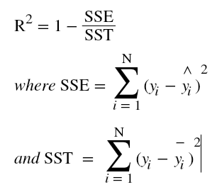
We define the error as the difference between the actual value of y and the predicted value of y. This error is calculated for every observation and thus can be positive or negative. Thus, squaring of each error is done to overcome the problem of cancellation of positive values with negative values of errors upon addition.

Coming back to our previous question, we follow the method of least squares to find the line of best fit.

Now, we have two equations and two unknowns, m and c. Solving the above two equations will result in those values of m and c which will give us an optimal solution and hence the equation for line of best fit.

or 

Moore’s law and Linear Regression

Sometimes we encounter some problems that do not seem to be linear at first. The relation between them can be exponential and thus non-linear. In such a case, it is required to convert those non-linear problems into linear problems and then find out the ‘Line of best Fit”.

Let’s take the example of a transistor. Transistor count on integrated circuits doubles every 2 years. Thus, the relationship between y and x comes out to be

where a is the default value or a constant. To make this equation linear, all we need to do is to take log on both the sides. The equation thus formed is

which is linear.

The Concept of R Squared

R Squared tells us about how much variation in  is explained by x_i in our model. R squared generally varies between 0 to 1 with the value of R squared equal to 1 signifying that our model is very accurate and 0 meaning model is very bad.

 

Thus, if R squared = 1, we have SSE = 0 or a perfect model. If R squared = 0, we have SSE = SST or  = mean of . Thus, the model comes out to be very bad. If it comes out to be a negative value, then we can say that the predicted value is worse than model having R squared = 0.

With this I conclude this tutorial. Stay tuned for more informative tutorials.

 

Please Write Your Comments.

Thanks,

Rakesh Kumar